Examples
Example 1: Excitation and Precession of a Single Spin
Let us start with a simple example of an uncoupled spin, for which the DROPS display is equivalent to the well-known vector representation. Selecting selects a single-spin system. By default, the initial state is \(I_{1z}\) (representing “z magnetization”). The red vector in the transparent red sphere should point along the z axis:

Fig. 184 \(\rho_0 = I_{1z}\)
By default, initially, the single spin is seen approximately from the positive z axis, dragging upward results in, for example, the view in Figure Fig. 185. You can manipulate the 3D display directly. Use one finger or the mouse to rotate the display like a trackball, or two fingers to pinch-zoom and rotate. For more information, see Manipulating the DROPS Display.

Fig. 185 Rotated view
E1 Display Operator
In order to see the currently displayed product operator, select .
As shown below, the list of product operators representing the current state contains only the term z, corresponding to \(I_{1z}\). Its coefficient has no imaginary part and the real part is 1.
(If a different initial state is shown, select .)

Fig. 186 \(\rho_0 = I_{1z}\)
E1 Edit Sequence
Also by default, the pulse sequence should be a 90°y pulse followed by a delay of 100 milliseconds. The pulse sequence is displayed schematically at the bottom of the screen. The 90°y pulse is represented by a yellow rectangle.
In order to see the detailed parameters of the currently selected pulse sequence, select . This displays the editable list shown in Figure Fig. 187. As expected, it consists of two elements: A 90°y pulse followed by a delay of 100 milliseconds. If a different pulse sequence is listed, select .

Fig. 187 The sequence editor
E1 Change Spin Params
By default, the offset frequency of the spin I1 is ν1 = 1 Hz. This can be checked (or modified) by selecting .

Fig. 188 \(\rho_0 = I_{1z}\)
The displayed parameter and its current value is indicated above the slider: “v1 = 1.00 Hz”.
E1 View Simulation
Pressing the play button at the bottom of the screen starts the simulation of the pulse sequence, and immediately shows the effects on the state. The pulse flips the spin by 90° around the y axis from z to x. During the delay, the spin rotates (precesses) around the z axis. The current time point is indicated by a circle and a vertical line.

Fig. 189 \(\rho_0 = I_{1z}\)
At the end of the sequence, the spin points along the x axis. As described in more detail in the Tutorial, the buttons at the bottom of the screen allow you to interactively control the simulation. For example, you can slow down or speed up the simulation or run the simulation in a loop. After stopping or pausing the simulation, you can change the current time point by moving the time cursor.
E1 View Param Changes

Fig. 190 \(\rho_0 = I_{1z}\)
You can also change the offset frequency (i.e. the rotation frequency during the delay) interactively while the simulation is running and immediately see the effect of the parameter change. Here, for \(v1=0.2 Hz\), the magnetization vector at the end of the delay points closer to the x axis than was the case with \(v1=1 Hz\).
Note
In this simple example, you learned how to define a spin system, the spin system parameters, the initial state, the pulse sequence and how to run and control the simulation. As we considered a single, uncoupled spin, the spin dynamics can be completely described by the well-known vector representation. In addition to the “magnetization vector”, the corresponding single-spin droplet (consisting of a red and green sphere) of the DROPS representation was displayed. Although this did not provide any additional information in this case, it is interesting to note that at all times, the magnetization vector is parallel to the corresponding droplet, i.e. to the axis formed by the centers of the green and red spheres. Hence, for the simple case of an uncoupled spin 1/2, the vector picture can be viewed as a special case of the DROPS representation. However, in contrast to the vector picture, the DROPS representation is not limited to uncoupled spins.
E1 Further Exploration
Suggestions for further exploration:
Predict the effect of the pulse sequence for different initial states and check your prediction by running the simulation.
Examples:
Observe the effect of the pulse sequence for the initial state \(I_{1x}\) rather than \(I_{1z}\).
Observe the effect of the pulse sequence for the initial state \(I_{1y}\).
What is the effect of the phase and/or flip angle of the excitation first pulse is modified?
Selecting provides the Sequence List, which in this case consists of two sequence elements: (1) The pulse 90°y and (2) the Delay 100 ms. If you double tap on 90°y, a sub menu opens in which you can change the flip angle and the phase of the pulse. In most cases, the pulses of interest will be 90° or 180° pulses, which can be chosen directly. If you would like to change the 90°y pulse e.g. to a 45°y pulse, select Other Pulse and enter the desired flip angle in the number pad.
Example 2: Rotation of \(I^+\) Around the z Axis
In this example, we use the SpinDrops app to visualize the droplet of the +1-quantum coherence term \(I_{1}^{+} = I_{1x} + i I_{1y}\) and to see its evolution under z rotations. Choose and select . For the sequence, select To see the corresponding Cartesian product operators, select

Fig. 191 \(\rho_0 = I_{1}^{+}\)
The left column of the list indicates the operator terms using the short-hand three-letter code (Cartesian Basis). On the right, the real and imaginary parts of the corresponding coefficients are displayed, which in general can be complex.
E2 The Droplet
In the vector picture, the state \(I_{1}^{+} = I_{1x} + i I_{1y}\) is represented by two vectors: A real vector (red) pointing along the x axis and an imaginary vector (yellow) pointing along the y axis.
|
= |
|
+ |
|


The corresponding droplet is a combination of the droplet for the operator \(I_{1x}\) (consisting of a red and a green sphere) and the droplet for the operator \(i I_{1y}\) (consisting of a yellow and blue sphere).
E2 Progression
As the sequence progresses over time, the \(I_{1}^{+}\) droplet will rotate around the z-Axis.
|
|
|
|
|
\(0°_z\) |
\(90°_z\) |
\(180°_z\) |
\(270°_z\) |
\(360°_z\) |
*I1p")
*I1p")
*I1p")
*I1p")
E2 Further Exploration
Suggestions for further exploration:
Observe the effect of the z rotation for different initial states, such as \(I_{1}^{-}\) or \(I_{1x}\).
Apply different rotations (e.g. around the x or y axis) using pulses.
Example 3: Weak Coupling Evolution in a Two-Spin System
Select and choose \(I_{1x}\) as the initial state by selecting . Select . In double tap the delay and set it to \(2 s\). Change the spin system parameters to v1=0 Hz, v2=0Hz, J12=1 Hz (if the parameter window is not visible, select ).

Fig. 192 \(\rho_0 = I_{1x}\)
Push the play button to run the simulation.
Initially, the droplet representing the linear spin operators of I1 shrinks and a new droplet emerges between I1 and I2, corresponding to the antiphase operator \(2I_{1y}I_{2z}\) (confirm using or using the right-hand rule). After 0.5 seconds (corresponding to \(1/(2 J12)\), the I1 spin droplet has completely vanished and the bilinear \(\{I1,I2\}\) droplet has reached its maximum size.

Fig. 193 \(\rho_0 = I_{1x}\)
E3 Evolution

Fig. 194 \(\rho_0 = I_{1x}\)
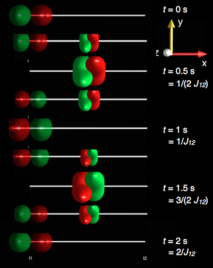
After 1 second (corresponding to \(1/J12\)), the \(\{I1,I2\}\) droplet vanishes and the I1 droplet reaches its maximum size again. However, notice that the sign of the I1 droplet (and of the magnetization vector) is inverted compared to the initial state at \(t = 0 s\). After 2 seconds (corresponding to \(2/J12\)), the initial state \(I_{1x}\) is reproduced. If the simulation is set to repeat mode, this will result in a continuous oscillation between the two droplets.
This simulation visualizes the well-known evolution of \(I_{1x}\) in the presence of a J coupling (in the weak coupling limit), which is given by \(I_{1x} cos(π J_{12} t ) + 2I_{1y}I_{2z} sin(π J_{12} t)\). For \(J_{12} = 1 Hz\) and \(t = 0.5 s\), the argument \((π J_{12} t ) = π/2\), i.e. the state is given by \(I_{1x} cos (π/2) + 2I_{1y}I_{2z} sin (π/2) = 2I_{1y}I_{2z}\). For \(t = 1 s, 1.5 s\), and \(2 s\), the state is \(-I_{1x}\), \(-2I_{1y}I_{2z}\), and \(I_{1x}\), respectively.
E3 Further Exploration
Suggestions for further exploration:
What happens if the offset frequency v1 is set to non-zero values?
What is the effect if the offset frequency v2 is set to non-zero values?
What happens if the initial state is \(I_{1z}\)?
Example 4: Refocusing of Offset and Coupling Effects
In this example, we illustrate the effect of 180° pulses on the evolution of a two-spin system. Select and set \(J_{12} = 1 Hz\) using the parameter slider (in ).

Fig. 195 t=0¶ |

Fig. 196 t=0.25¶ |

Fig. 197 t=0.5¶ |
We consider the evolution of the initial state \(I_{1x}\) (select ) during a delay \(T = 1/(2 J_{12}) = 0.5 s\) (select .
The panels above show the DROPS visualization of the system at \(t = 0 s\), \(t = 1/(4 J12) = 0.25 s\), and \(t = 1/(4 J12) = 0.5 s\), for the case where both offset frequencies are zero (ν1 = ν2 = \(0 Hz\)).
In this case, initial x magnetization of the first spin (\(I_{1x}\)) evolves under the weak coupling Hamiltonian during the delay \(T = 1/(2 J12)\) completely to the anti-phase operator \(2I_{1y}I_{2z}\). In the following, we simulate the resulting final state without and with additional 180° pulses in the center of the delay T, assuming a non-zero offset frequency of the first spin (\(ν1 = 0.5 Hz\)).
E4 Refocusing of Offset Effects
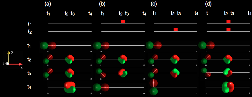
For \(ν1 = 0.5 Hz\) and \(J12 = 1 Hz\), simulations are shown for \(t1 = 0 s\), \(t2 = T/2\) = \(1/(4 J12)\) = \(0.25 s\), \(t3 = t2\) (assuming a negligible duration of the 180° pulses) and \(t4 = T = 1/(2 J12) = 0.5 s\).
\(I_{1x}\) evolves
to \(-2I_{1x}I_{2z}\) in the absence of pulses during the delay T,
to \(I_{1x}\) if a spin I1-selective 180°x pulse is irradiated at T/2,
to \(I_{1y}\) if a spin I2-selective 180°x pulse is irradiated at T/2,
to \(2I_{1y}I_{2z}\) if I1- and I2-selective 180°x pulses are irradiated at T/2.

Fig. 198 [click to try (d) interactively in another window]
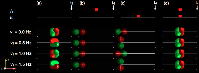
These results reflect the well-known fact that in case
offset and coupling terms of the Hamiltonian are active.
the effect of the coupling and of the offset ν1 are refocused.
the effect of the coupling and of the offset ν2 are refocused but ν1 is active.
the simultaneously irradiated I1- and I2-selective 180°x pulses at T/2 (corresponding to a non-selective 180°x pulse for the two-spin system) refocus frequency-offset effects but the coupling evolution is active. For the initial state \(I_{1x}\), this is confirmed by the resulting final state of the system at t4 = T = 1/(2 J12) = 0.5 s for different offsets ν1 of 0 Hz, 0.5 Hz, 1 Hz and 1.5 Hz.
E4 Further Exploration
Suggestions for further exploration:
Does the offset ν2 of the second spin have any effect in the experiment from the example? What if we start with the initial state \(I_{2x}\) instead of \(I_{1x}\)?
How would the results change if 180°y pulses rather than 180°x pulses were used in the example?
Explore the effects of selective and non-selective 180° pulses in three-spin systems.
Explain the results of the refocusing experiments using the product operator formalism.
Example 5: Spectral Editing
The DEPT experiment (Distortionless Enhancement of Polarization Transfer) makes it possible to distinguish C, CH, CH2, and CH3 groups. The 1H spins are excited and the amplitude and sign of the detected 13C spin depends on the number of attached protons.
The basic pulse sequence of the DEPT experiment has the form
90°x(H) - T - 180°x(H),90°x(C) - T - θ y(H),180°x(C) - T
where the flip angle \(θ\) of the editing 1H pulse is 45°, 90° or 135° and the delay T is \(1/(2 J_{CH})\). The experiment relies on polarization transfer so that only signal originating from 1H polarization is detected on the 13C frequency. Hence, the spins of 13C atoms without attached 1H atoms do not yield any detectable signal. Predicting the 13C signals of CH, CH2, and CH3 is less simple.
As up to three spins 1/2 can be considered in the current version of SpinDrops, it is only possible to simulate the relative size and sign of of the final 13C magnetization for CH and CH2 groups (and hence of the relative size and sign of the corresponding 13C NMR signal), but not yet CH3. In the following, we will assume that spin I2 represents a 13C spin and spins I1 and I3 represent 1H spins:
CH system |
with J12 ≠ 0 |
|
CH2 system |
with J12 = J23 ≠ 0, and J13 = 0. |
E5 DEPT-45
Select . To simulate the CH system, set J12 = 1 Hz, J13 = 0 Hz, and J23 = 0 Hz () and define the initial state as \(I_{1z}\) (Initial Selecting ). For the CH2 system, set J12 = 1 Hz and J23 = 1 Hz and define the initial state as \(I_{1z}+I_{3z}\) (). Select and run the simulation. Notice that in both cases the final magnetization vector of spin I2 is pointing in the positive x direction.

Fig. 199 DEPT-45 \(CH\) : J12 = 1 Hz

Fig. 200 DEPT-45 \(CH_2\) : J12 = 1 Hz, J23 = 1 Hz
E5 DEPT-90
Select and run the simulation. Note that compared to the DEPT-45 sequence shown on the previous page, the flip angle \(θ\) of the editing pulse has changed from 45° to 90° (the yellow pulses).
In DEPT-90, the final magnetization vector of spin I2 is pointing in the positive x direction for CH (orange ellipse). However, for CH2 the final magnetization vector of spin I2 is zero (orange ellipse). This results in positive 13C-NMR signals for CH groups but no 13C-NMR signals for CH2 groups.

Fig. 201 DEPT-90 \(CH\) : J12 = 1 Hz

Fig. 202 DEPT-90 \(CH_2\) : J12 = 1 Hz, J23 = 1 Hz
E5 DEPT-135
Selecting changes the flip angle θ of the editing pulses to 135°.
In this case of DEPT-135, the final magnetization vector of spin I2 is pointing in the positive x direction for the CH system, whereas it is pointing in the negative x direction for the CH2 system. This results in positive and negative 13C-NMR signals for CH and CH2 groups, respectively.

Fig. 203 DEPT-135 \(CH\) : J12 = 1 Hz

Fig. 204 DEPT-135 \(CH_2\) : J12 = 1 Hz, J23 = 1 Hz
E5 Further Exploration
Suggestions for further exploration:
What are the expected relative signal amplitudes for CH and CH2 groups in DEPT-45, DEPT-90 and DEPT-135? (Tip: Remember that you can always display the coefficients of the product operator terms by selecting )
Does the final DROPS display (and hence the final state of the spin system) depend on the offset frequencies ν1, ν2, ν3?
Which product operator terms are created at the end of DEPT-45, DEPT-90, and DEPT-135 in addition to the desired magnetization of spin I2?
Calculate the effect of the DEPT experiments analytically using the standard product operator formalism and compare the results with the DROPS simulations. What are the expected relative signal amplitudes for CH3 groups in DEPT-45, DEPT-90 and DEPT-135?
Example 6: TOCSY Transfer in a Two-Spin System
In this example, we explore the transfer of x magnetization in the isotropic mixing period of TOCSY experiments, where isotropic mixing conditions are created by a multiple-pulse sequence. Select and choose \(I_{1x}\) as the initial state by selecting . Choose the isotropic mixing sequence for two spins by selecting .

Fig. 205 Before isotropic mixing
The isotropic mixing period is indicated by a grey rectangle. Set the coupling J12 to 1 Hz. (Here, the offset frequencies v1 and v2 are irrelevant as they are effectively suppressed by the isotropic mixing sequence.) Interestingly, after 0.5 seconds, corresponding to \(t = 1/(2 J12)\), the initial state \(I_{1x}\) has turned completely into \(I_{2x}\), i.e. x magnetization has been fully transferred from the first to the second spin).

Fig. 206 After isotropic mixing
E6 TOCSY Transfer Return
Under the isotropic mixing Hamiltonian, the initial state
Creating a circulation like:
This can be verified by using Figure Fig. 207 as a
starting point, and extending the duration of the isotropic mixing
period to \(1 s\) (or more, by selecting , double tapping Hiso12, and changing
the pulse length from 0.5/J12 to 1/J12.)

Fig. 207 Change the pulse length here
For \(t = 1/(4J12)\) (corresponding to \(t = 0.25 s\) for \(J12 = 1 Hz\)), the argument \((π J_{12} t) = π J_{12}/(4J12) = π/4\) and \(\cos(π J12 t ) = \sin(π J12 t ) = \frac{1}{\sqrt 2}\). Hence the state is \(0.5 I_{1x} + (I_{1y}I_{2z} - I_{1z}I_{2y}) + 0.5 I_{2x}\) and the bilinear droplet located between I1 and I2 reaches its maximum value.
For \(t = 1/(2J12) = 0.5 s\), \((π J12 t ) = π J12/(2J12) = π/2\) and \(cos(π J12 t ) = 0\), \(sin(π J12 t ) = 1\). Hence, the state is \(I_{2x}\), i.e. the initial x magnetization has been fully transferred from spin \(I_1\) to spin \(I_2\). For \(t = 1/J12 = 1 s\), the state is again \(I_{1x}\) and the cycle starts anew.
Example 7: Inversion of Multiple-Quantum Coherence
In the standard SpinDrops representation, a non-selective 180°y pulse simply rotates the droplets by 180° around the y axis. This is illustrated here for the initial operator \(I_{1}^{+}I_{2}^{+}I_{3}^{+}\)
(select ).

Fig. 208 \(\rho_0 = I_{1}^{+}I_{2}^{+}I_{3}^{+}\)
In addition to the initial orientation of the droplet, the snapshots show its orientations after rotations of 45°, 135°, and 180° around the y axis.

Fig. 209 0°¶ |

Fig. 210 45°¶ |

Fig. 211 135°¶ |

Fig. 212 180°¶ |
The fact that this operation also inverts the coherence order from \(p=+3\) to \(p=-3\) can be inferred from the direction of the rainbow colors of the initial and final droplet orientations. However, this can be seen more directly by separating the droplet according to coherence order \(p\):
In the previous examples, the Standard Plane display mode was selected. To separate the droplets according to coherence order \(p\), choose . In this display mode, the change of coherence order from \(p=+3\) to \(p=-3\) (via all the intermediate coherence orders) can be clearly followed. In Coh. Order p display mode, the droplets are arranged in planes with coherence order \(p=3\) at the top and \(p=-3\) at the bottom, as explained in DROPS Representation. The black triangle in the center corresponds to \(p=0\).

Fig. 213 \(\rho_0 = I_{1}^{+}I_{2}^{+}I_{3}^{+}\)
E7 Further Exploration
Suggestions for further exploration:
Study the effect of pulses and delays on various initial states of pure or mixed coherence orders.
Test the different display modes with droplet separations based on coherence order \(p\), the absolute value of coherence order \(|p|\) and/or tensor rank \(j\).